Turbulence is a crucial part of the climate, the dynamo process by which the Sun and Earth produce magnetic fields, and a major limiting factor for plasma confinement in tokamaks. In each of these systems, the largest scales are factors of 105 to 1014 times larger than the smallest scales. Crucially, energy flows through all of these scales, impacting the dynamics of the flow. A complete numerical simulation would require between 1015 to 1042 data points for every moment in time simulated! This is…not quite feasible. One of the particularly interesting questions in out-of-equilibrium systems is how often extreme events occur. They are rare, but how rare? What are the statistics of these flows?
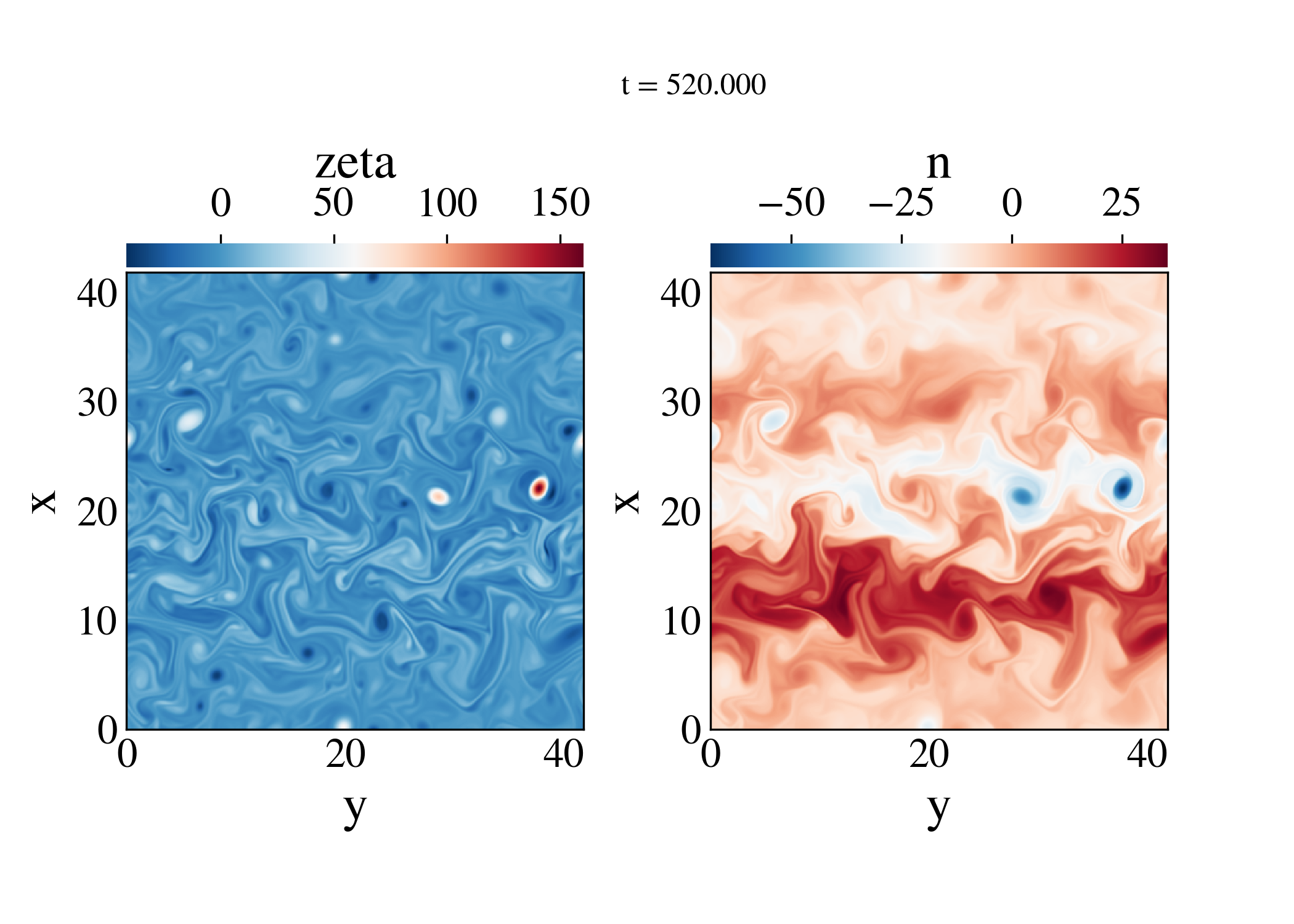
We are particularly interested in systems with some form of anisotropy: a preferred direction, which may be imparted by rotation, a strong magnetic field, or a combination of both. In such systems, in addition to energy flowing from large scales to small (or vice versa, in the case of two-dimensional flows), there are often the formation of large scale structures, typically called zonal flows or jets. You can see one example of this in the image above. The right hand panel shows the plasma density in a simplified model of tokamak turbulence called the modified Hasagawa-Wakatani system. You can see that the system is forming large, coherent structures in the y direction. These are zonal flows.
Instead, we work on developing models and approximation techniques to reduce the amount of data we need to store to faithfully recreate the dynamics. We can think of the state of the system as a single point in a 1042 dimensional space evolving in time. Using this idea, we can imagine projecting onto a lower dimensional space while still maintaining the time history of the state.
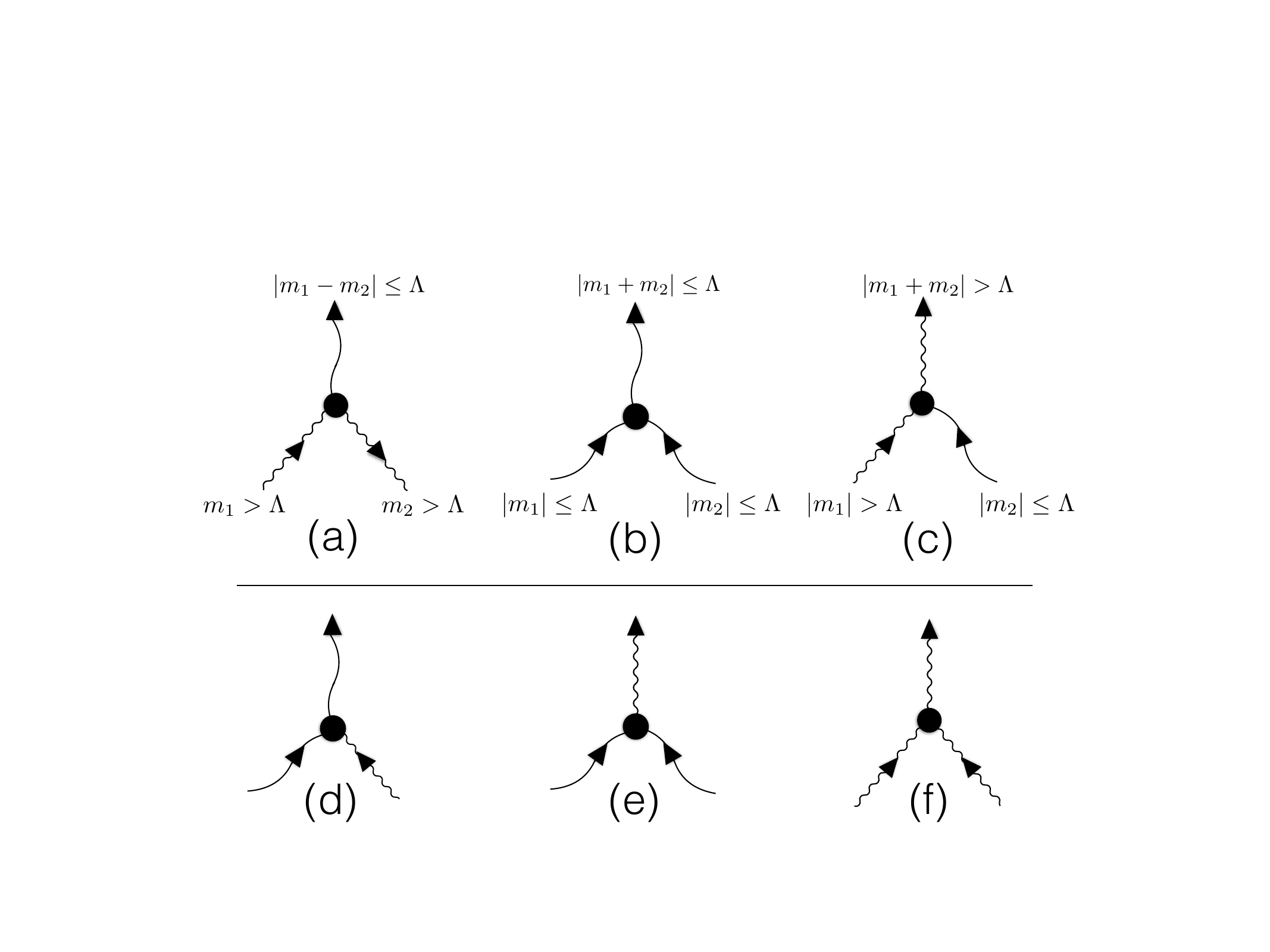
We’re particularly interested in the Generalized Quasilinear Approximation (GQL) and Direct Statistical Simulation. GQL works by decomposing the state vector $\mathbf{X} = \mathbf{X}_l + \mathbf{X}_h$ into low and high wavenumbers. In the figure above (courtesy of Brad Marston), the top row shows non-linear interactions preserved by GQL and the bottom row shows those it eliminates. $\Lambda$ is the wavenumber delineating low and high.
We’ve used GQL to study the Busse annulus. Recently, group alum Morgan Baxter wrote some new tools to easily implement GQL in Dedalus. We are currently trying them out on many classic flows including Taylor-Couette, Rayleigh-Benard Convection, and the thermal asymptotic suction boundary layer.
More about DSS can be found here.